| Matheus Belucio1; José Alberto Fuinhas2; José Antunes3; Victor Sá4; Joana Mota5. |
| 1 - CEFAGE-EU, Department of Economics, University of Évora and Faculty of Economics, University of Coimbra; Colégio do Espírito Santo, Largo dos Colegiais, 2, 7000-803, Évora, Portugal. |
| 2 - NECE-UBI and CeBER, Faculty of Economics, University of Coimbra, Portugal. |
| 3 - University of Beira Interior, Portugal. |
| 4 - University of Porto, Portugal. |
| 5 - University of Minho, Portugal. |
Abstract
The gambling expenditure in the United States have been analysed for the period from 1965 to 2016. The effects of income, misery index, electricity consumption, population growth on gambling expenditure were analysed through an ARDL model. The method that deals well with the autoregressive nature of the phenomenon. The results support that gross domestic product has an impact on gambling expenditure in both the short- and long-run. While the misery index (or its decomposition) only has an effect in the long-run. The consumption of electricity that was used as a proxy for new forms of gambling is related to gambling expenses. It suggests that new forms of gambling can be a risk to the gaming industry in long-run. Our results show the economic outlook on the phenomenon of gambling. It presents useful information to public policymakers and the gambling industry and contributes to the literature on the phenomenon of gambling.
Keywords: Gambling Expenditure; United States; ARDL model.
JEL Classification: L83; C51; P36.
Resumo
As despesas com jogos de azar nos Estados Unidos foram analisadas para o intervalo de tempo entre 1965 e 2016. Os efeitos da renda, do índice de miséria, do consumo de eletricidade e do crescimento populacional nas despesas com jogos de azar foram analisados com o modelo ARDL. O método lida bem com a natureza autoregressiva do fenômeno do jogo. Os resultados confirmam que o Produto Interno Bruto tem impacto nas despesas com jogos de azar tanto a curto como a longo prazo. Enquanto o índice de miséria (ou a sua decomposição) só tem um efeito de longo prazo. O consumo de eletricidade que foi usado como proxy para novas formas de jogo e provou que está relacionado com as despesas efetuadas com os jogos de azar. Isso sugere que as novas formas de jogo podem ser um risco para a indústria de jogos no longo prazo. Os resultados mostram que a perspectiva econômica deve ser considerada quando se analisa o fenômeno do jogo. De facto, os fenômenos econômicos têm informações úteis para os decisores de políticas públicas e também para a indústria do jogo. Além de interagir com a literatura de diversas áreas sobre o fenômeno do jogo.
Palavras-chave: Despesas com jogos de azar; Estados Unidos; Modelo ARDL.
JEL Classification: L83; C51; P36.
1 - INTRODUCTION
It is commonly perceived that economists’ work is directed towards understanding social and economic phenomena. However, since it is a social science, economics focuses on the study of individuals and their interactions. Considering that gambling is an interaction between individuals and groups in a specific society, the economic analysis could contribute by providing new tools and data for public and private decision making.
The gambling phenomenon is found in both rich and developing countries alike, which indicates that it is a natural human action. Several historical examples show the presence of gambling when economies are at their peak. The objective of this study is to analyse, from an economic point of view, the phenomenon of gambling expenditure.
Gambling is a popular activity that has been part of most cultures over the centuries (McMillen, 2005; Bernstein, 1996) and leads individuals to take a risk in pursuit of something more valuable voluntarily. The game is a way to achieve the excitement (American Psychiatric Association, 2014). Moreover, the belief that money is both a cause and solution to problems is a characteristic commonly found in gamblers (American Psychiatric Association, 2014).
The advent of online gambling opened new frontiers and brought new age groups, increasing the overall size of the market. More specifically, the American Gaming Association (AGA) is the most significant group representative of the U.S. casino industry totalling 240 billion dollars. This industry spreads across forty states and represents 1.7 million jobs (AGA, 2017). In Las Vegas (which is the major gambling city in the U.S.A.), for the period from 2001 to 2016, the total gross domestic product doubles in value $55535 to $111091 millions of dollars (FRED, 2017).
The use of econometrics makes it possible to analyse, in a practical way, the social phenomena; its interpretation gives robustness to the discussion. Therefore, after performing several tests and diagnostic statistics that allowed us to identify the nature of the variables, we selected the ARDL model that allows understanding the long- and short-run relationships (the time horizon studied was from 1965 to 2016), to answer the question of research “Does the economic situation influence expenses with gambling?” The hypotheses raised for this study are:
The independent variable ‘personal expenditure with gambling’ does not present any specifics. Nothing suggests it is restricted to the casino or even to other forms of gaming, ignoring forms (such as Native American gaming) that mostly take place regionally. In other words, it seems to capture the spending with the entire sector annually.
The misery index of the United States was calculated and used; the variables that compose the index (inflation and unemployment) were also used to give robustness to the results of the model. Along with the GDP, it is an excellent way to get a grasp on the financial situation of the people. Energy consumption was used as a proxy for new forms of play and the population as a control variable.
Our results suggest that GDP shows an impact on both short- and long-run on gambling expenditures. Besides, the misery index, the unemployment and the inflation only impact in the long-run. Other economic policymakers and players might find this article useful, as it includes a new view of the relationships of gambling and society.
The paper was organised in five different sections. The first one presents an introduction to the gambling phenomenon and its background; the second one develops the debate regarding the literature and is followed by methodology. The fourth section presents the results and discussion, and finally, the conclusion.
2 - LITERATURE REVIEW
Several historical reports confirm that humankind has been involved with gambling (McMillen, 2005; Barbieri, 1999). Throughout history, more prosperous societies (Roman, Greek, Egyptian, and currently American) have had a connection with different forms of games. Gambling is understood as an activity that is not harmful to some, meanwhile, for others is very damaging (George et al., 2017). If one considers the rationality of individuals, then gambling is a voluntary action that involves risk, and its objective is the economic gains (Beyerlein & Sallaz, 2017).
Fiedler et al. (2019) showed that pathological gambling – which accounts for a significant portion of revenue in the industry – leads to high social costs and also suggested that income inequality might be related to spending concentration. Problematic gamblers also face new risks, such as cryptocurrencies (Mills & Nower, 2019).
Van den Bergh (2009) joined opinions from various prestigious economists over GDP. They consider the GDP the best indicator to measure economic activity and social welfare. Dolan (2008) states that the fact that several discussions exist contributes to economists and psychologists to have a better understanding of the determinants associated with well-being. Indeed, it is possibly to relate wealthier economies with higher incomes (Howarth & Kennedy, 2016; Kahneman et al., 2006).
Frequently, economic growth-energy nexus is the object of study (e.g. Marques et al., 2017; Choi et al., 2017; Rahman et al., 2017; Lai et al., 2011). Fuinhas et al. (2015) highlight that variables which measure electrification can be used as a proxy of economic development. However, more energy consumption will possibly imply more adverse impacts on the environment. Li et al. (2014) found evidence that in the case of Macau, that hypothesis is correct, as it has contributed to provoking more CO2 emissions.
Marques et al. (2017) point out that economic and social globalisation has a relationship, in the same way, with economic growth and energy consumption. Simcock & Mullen (2016) sustain that contemporary societies require the usage of electricity in domestic life. Choi et al. (2017) found that the relative energy intensity could lead to an increase in the companies’ profitability. The gambling industry is significant in the American economy. Therefore, economic variables (such as GDP and electricity consumption) could also have explanatory power over gambling expenditures. We are going in with the results obtained by Lai et al. (2011) for Macau, another world centre of gambling.
In the next subsection, we will approach the methodology and the data utilised to quantify the impacts of gambling in the US economy.
2.1 Gambling
The literature on gambling in the USA is vast. This literature discusses several gambling effects over a wide range of fields such as tourism, and health (psychiatry/psychology). In table 1 presents the main literature’s highlights.
Table 1 - Current literature on gambling.
| Authors | Highlights |
|---|---|
| Gu et al. (2017) | Adequate regulation and public intervention are required to maximize benefits. |
| Guo et al. (2017) | Gambling acts as a tourism enhancer in both Mississippi and Alabama. |
| Akee et al. (2015) | Effects on American Indian economic development. |
| Nichols et al. (2015) | Fiscal impacts of legalised casino gambling. |
| Horváth & Paap (2012) | The gambling industry is essential in the US. |
| Hofer & Leitner (2011) | In their proposed model the European lotteries are less profitable than the American ones. |
| Walker & Jackson (2010) | Types of gambling that promote tourism have a stronger influence on state tax revenues. |
Source: Author’s elaboration.
It is essential to weigh the different aspects of gambling in order to promote debate. There is also much discussion in literature over the impacts of gambling; the results of various researches show positive and negative effects, as can be seen in table 2.
Table 2 - Literature on how gambling affects society.
| Authors | Positive | Negative |
|---|---|---|
| Nichols & Tosun (2017) | Indian casinos associated with a significant decrease in crime in neighbouring counties. | After the opening of a new casino, there is a surge in crime in the short-run. |
| AGA (2017) | The casino supports 350000 small business jobs. | - |
| Davis et al. (2017) | - | There was a presence of gambling disorders among the USA veterans. |
| Akee et al. (2015) | Fiscal Independence; Social and economic development. | - |
| Nichols et al. (2015) | Small economic impact | - |
| Horváth & Paap (2012) | An important role in state revenue | - |
| Li et al. (2010) | Casinos can attract foreign visitors. With adequate strategy, the trade can be maximised. | - |
| Dadayan & Ward (2009) | During the crisis, states look to increase gambling revenue to balance the budget. | - |
Source: Author’s elaboration.
A country, state or city government may find on gambling legalisation a vital revenue stream. As seen in Macau, taxation on the gambling industry represented one of the primary sources of income for the government (Gu & Tam, 2011). Thanks to the gambling industry, other businesses are necessary. In areas where gambling is intrinsic to the population, companies in those regions usually invest more in research and development (Adhikari & Agrawal, 2016). Figure 1 resumes this subsection.
Figure 1 – Gambling industry and Society.
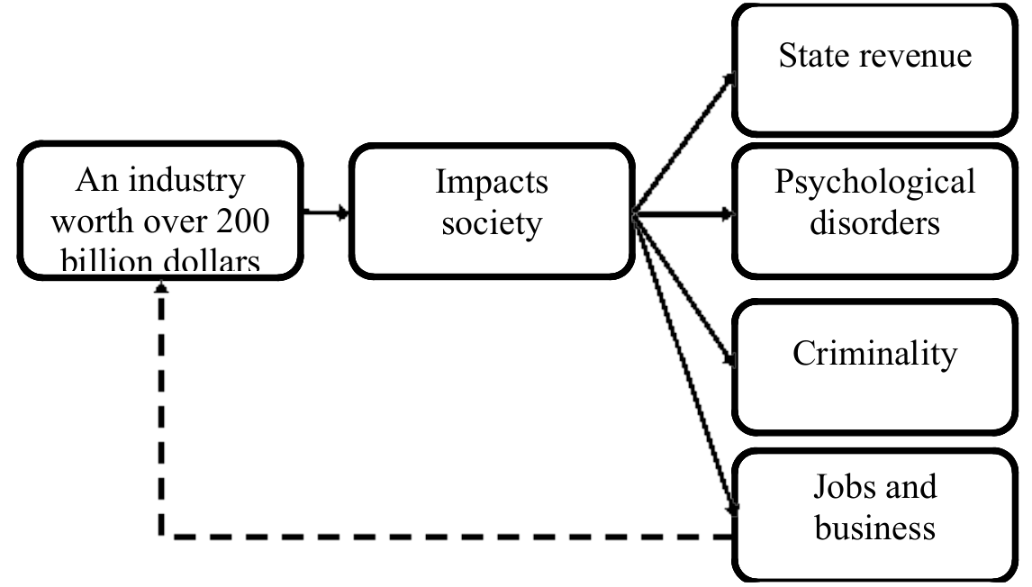
Source: Author’s elaboration.
In synthesis, the gambling industry must not be devalued, and its influence on the economy is of the utmost importance. One of the critical impacts in the local community is the business dynamic that the gambling industry creates, improving the economic well-being of the population.
2.2 Misery Index
Arthur Okun created the misery index in the ’70s. The index is built by adding the inflation and the unemployment rates. The index become famous thanks to its use as ammunition in political debates between candidates, in several US presidential elections (Lovell and Tien, 2000).
Empirical research reveals that higher rates of unemployment and inflation have economic and social costs for a country, which causes a decrease in the well-being of economies and their respective populations (e.g. Donayre & Panovska, 2018; Ahmad & Mykhaylova, 2017; Nucera, 2017; Ayllón & Ferreira-Batista, 2017).
Green (2011) argues that it is essential to understand the role of employability and its impacts when it comes to policies. Unemployment affects mental health in particular (Drydakis, 2015). Green (2011) also points out that an increase in unemployment causes a decrease in well-being.
Some of the criticism of the index was based on the fact that with only two variables being analysed it would lead to an excessive simplification of the economic reality (Lovell and Tien, 2000). Ramoni-Perazzi & Orlandoni-Merli (2013) discuss in their paper several formulations of the misery index and proposed a new version adding employment in the informal sector to the original model.
Barro (1999) proposed a new model, adding to the index the long-run interest rate as well as the GDP variation, which brought more credibility and explanation power to the index. Barro (1999) used it to compare the economic success of the US presidents’ mandates since 1949.
As far as we know, the first study connecting misery index and gambling can be attributed to Özcan & Açıkalın (2015). That study aimed to verify a causal relationship between the misery index and lottery games in Turkey. The index used in their research was a variation of the Okun’s index by adding the interest rate; they found a positive relationship between the variables.
It is common knowledge that misery can impact the decision-making process. Indeed, it is one reason that drives some individuals to risk everything they have, to achieve a “better” standard of living.
The United States had witnessed an increase in opportunities for gambling (Beyerlein & Sallaz, 2017), which was possible to observe at the end of the 20th century when gambling was becoming an everyday activity, and the industry was rapidly growing (National Gambling Impact and Policy Commission (US), 1999). In short, the misery index can be utilised as a tool for economic analysis, policy evaluation and well-being.
In the next section, we will approach the methodology and the data utilised to quantify the impacts of gambling in the US economy.
3 - METHODOLOGY
This section is devoted to the presentation of the econometric model used and the reasons for its choice. We also present the selected data and their characteristics. To finish, the way data and model relate and interaction to obtain empirical results.
3.1 ARDL model
Like all addictions, gambling is easy to access. However, the process of recovery is slow, painful and riddled with challenges. Relapses corroborate that addictive behaviour is autoregressive by default, which means that it has lasting effects on time, even when the nature of gambling is not constant.
In this study, we used a methodology that focuses on autoregressive phenomena: Autoregressive Distributed Lag (ARDL). Shin et al. (2014) developed a cointegrating nonlinear Autoregressive Distributed Lag, this is the extension of Pesaran et al. (2001) model, commonly called ARDL and widely used in the literature (e.g. Rahman & Kashem, 2017; Goh et al., 2017; Jalil et al., 2013; Fuinhas & Marques, 2012).
The use of this methodology allows studying the long and short-run effects of the independent variables on the dependent variable, which enables a more comprehensive analysis which results in more robust research. The long-run impacts can be studied due to the data spanning from 1965 to 2016, with a shorter period such an analysis would not be possible.
The ARDL models have the following structure:
Model I:
\[\Delta DLPC_{it} = \alpha_{1i} + \beta_{1i1} DLGDP_{it} + \beta_{1i3} DPOPG + \beta_{1i3} DPOPG_{it - 1} + \beta_{1i4} DLPC_{it - 1} + \delta_{1i}\qquad(1)\]
Model II:
\[\Delta DLPC_{it} = \alpha_{2i} + \beta_{2i1} DLGDP_{it} + \beta_{2i3} DLPOPG + \beta_{1i3} DLPOPG_{it - 1} + \beta_{2i4} DLPC_{it - 1} + \varepsilon_{1i}\qquad(2)\]
Firstly the \(\Delta DLPC\) is the vector of the dependent variable. The \(\alpha_{i}\) stands for the intercept, \(\beta_{i}\) and \(\delta_{i}\) represent the estimated coefficients, with \(n = 1, \dots, 5\), finally \(\varepsilon_{it}\) represents the term of error.
The ARDL model can still be developed with variables that have different orders of integration I (0) and I (1). It is essential to consider the results obtained with the autoregressive econometric model. Check the Error Correction Model (ECM) signal obtained from the Wald test (in case of negative value the model has a long-run explanation, through the elasticities).
3.2 Data
To test the relationship between gambling and misery index in the USA, we used the annual data from 1965 to 2016, for this time series there is no break in the data. The descriptive statistics were conducted on the raw variables, previous to any transformations, the stepping stone to the construction of the several models that we will present further down this paper. Afterwards, several transformations were made to the data creating the variables that were used in the models. In table 3 we present the descriptions of the variables, the database where they were obtained, transformations and the descriptive statistics.
Table 3 – Table 3 – Descriptive statistics, variables and databases
|
|
|||||
|---|---|---|---|---|---|
| Variable | Obs | Mean | Std. Dev. | Min | Max |
| lpc | 52 | 3.637 | 0.936 | 2.033 | 4.761 |
| lgdp | 52 | 9.203 | 0.348 | 8.547 | 9.736 |
| popg | 52 | 1.002 | 0.168 | 0.693 | 1.387 |
| lteri | 52 | 10.788 | 0.104 | 10.484 | 10.917 |
| infl | 52 | 4.050 | 2.836 | -0.356 | 13.509 |
| un | 52 | 6.102 | 1.625 | 3.500 | 9.700 |
| myi | 52 | 10.152 | 3.408 | 5.419 | 20.609 |
|
|
|||||
| Variables | Acronyms | Databases | Units | Transformations | |
| Consumer Price Index | CPI | AMECO | Index | Divided by 100 | |
| Population Growth | DLPOPG | Worldbank | Rate | - | |
| Personal Consumption Expenditures on Gambling | DLPC | FRED | Billions of Dollars | Divided by CPI | |
| Gross Domestic Product | DLGDP | FRED | Billions of Dollars | Divided by CPI | |
| Misery Index | DMYI | World Bank and Bureau of labour statisticIndex | Sum of inflation and unemployment | ||
| Inflation | DLAINFL | World Bank | Index | - | |
| Unemployment | DLAUN | Bureau of labour statistic | Index | - | |
| Total Energy Consumption | DLTERI | EIA | Trillion Btu | Sum of total energy consumption of Residential and Industrial Sectors. | |
Note: D and L denote first differences and natural logarithm, respectively; FRED: Federal Reserve Bank of St. Louis (https://fred.stlouisfed.org/series/DGAMRC1A027NBEA); EIA: Energy Information Administration (https://www.eia.gov/); AMECO: Annual macro-economic database of the European Commission’s Directorate General for Economic and Financial Affairs (https://ec.europa.eu/info/business-economy-euro/indicators-statistics/economic-databases/macro-economic-database-ameco_pt); Worldbank: World Development Indicators (https://databank.worldbank.org/data/reports.aspx?source=2&series=NY.GDP.MKTP.KN&country=#).
Source: Author’s elaboration.
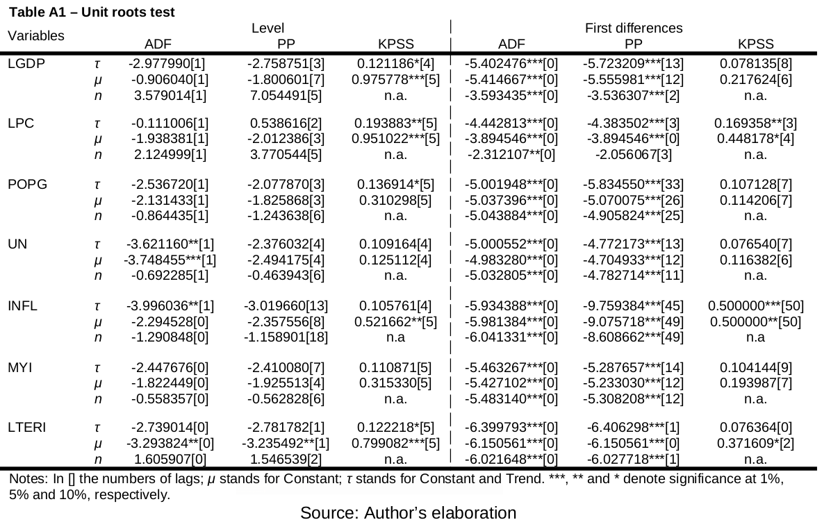
The study of the unit-roots allows us to understand the nature of the variables better. The order of integration of the variables must be either I(0) or I(1) in order to use the ARDL methodology (e.g. Shahzad et al., 2017; Sek, 2017; Chang & Chen, 2017; Katrakilidis & Trachanas, 2012; Marques et al., 2017). The unit-roots Augmented Dickey-Fuller (ADF) and Phillips–Perron (PP) test reveals the nature of series and allows excluding the variables being cointegrated of second-order (I(2)). For more details on stationarity, see table A1, which also presents the KPSS test.
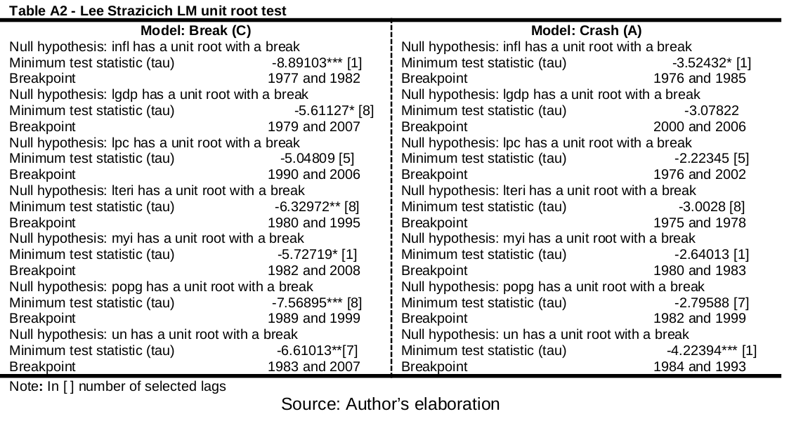
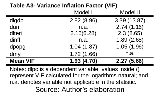
The breakpoint unit roots test was performed to detect the presence of structural breaks in the series, and several dates are suggested. Due to the number of observations, we use in the execution of the test, the Schwarz Information Criterion. The null hypothesis is the presence of unit root. For more details, see table A2. The Variance Inflation Factor (VIF) statistic confirms that the data is free from the menace of multicollinearity, which is required for the use of the proposed methodology, for more details see Table A3 (in the appendix). In the next section show the estimation ARDL model.
The variables above are related to the state of the American economy. The reason they were chosen was to demonstrate the impact of those macroeconomic indicators on the gambling industry.
According to the World Bank (2019), the GDP captures ‘the sum of gross value added by all resident producers in the economy plus any product taxes and minus any subsidies not included in the value of the products’. In this case, it is used to measure wealth in the USA. Inflation is supposed to show the differences in cost of living among the years.
That – along with unemployment – comprises the misery index, through which not only can we assess what the economic situation is like but also the true extent of poverty in the country. Likewise, population growth is related to social welfare.
Note that the consumer price index (CPI) was used to remove inflation from the variables gross domestic product (GDP) and personal consumption expenditures on gambling (PC). The study contains the maximum number of data available for the time-span in the study (52 years), it is worth observing that the longer the time horizon of the series, more robust is the estimation (Fuinhas & Marques, 2013).
The data presented above is the stepping stone used in the construction of the econometric models. The tests performed up to this point allow us to continue to follow the proposed methodology. In section 5 we will present the empirical results.
4 - RESULTS AND DISCUSSION
In this section, we will present the results of the study, as well as the diagnostic tests of the robustness of the estimation, also making a brief discussion about the phenomenon.
We start by presenting the result of the Dumitrescu & Hurlin (2012) causality test that also allows the capture of the relationship between the variables through a pair structure. Table 4 shows the results.
Table 4 – Dumitrescu & Hurlin (2012) causality test.
| 1 lag (51 observations) | 2 lags (50 observations) | |||
|---|---|---|---|---|
| F-Statistic | Prob. | F-Statistic | Prob. | |
| UN does not Granger Cause LPC | 3.6774 | 0.0611 | 2.6975 | 0.0783 |
| LPC does not Granger Cause UN | 0.0741 | 0.7866 | 0.7342 | 0.4856 |
| LTERI does not Granger Cause LPC | 1.1398 | 0.2910 | 0.6190 | 0.5430 |
| LPC does not Granger Cause LTERI | 2.3827 | 0.1293 | 2.1533 | 0.1279 |
| INFL does not Granger Cause LPC | 0.0026 | 0.9598 | 1.0873 | 0.3458 |
| LPC does not Granger Cause INFL | 5.6368 | 0.0216 | 4.7967 | 0.0129 |
| LGDP does not Granger Cause LPC | 7.2561 | 0.0097 | 2.1373 | 0.1298 |
| LPC does not Granger Cause LGDP | 5.2182 | 0.0268 | 2.9711 | 0.0614 |
| POPG does not Granger Cause LPC | 6.1416 | 0.0168 | 2.7298 | 0.0760 |
| LPC does not Granger Cause POPG | 0.4514 | 0.5049 | 0.6376 | 0.5333 |
| MYI does not Granger Cause LPC | 0.8445 | 0.3627 | 0.8173 | 0.4481 |
| LPC does not Granger Cause MYI | 3.7587 | 0.0584 | 2.2509 | 0.1170 |
Source: Author’s elaboration.
All variables have some relation to gambling expenses. The only exception is the LTERI variable that is not directly related to gambling expenses. That result was not surprising, but its relationship is interacting with other variables in the model is expected as it acts as a proxy. Thus, this fact does not negate its use. The highlight of this test is for the GDP with the use of 1 lag presented bidirectional relationship with gambling expenses.
In the ARDL models (see table 5), the dependent variable used is the first differences of LPC.
Table 5 –ARDL results.
| Model I | Model II | |
|---|---|---|
| Short-run | ||
| DLPC(-1) | 0.271453\(\ast\ast\ast\) | 0.294237\(\ast\ast\ast\) |
| DLGDP | 1.011477\(\ast\ast\ast\) | 1.070884\(\ast\ast\ast\) |
| DPOPG | 0.103208\(\ast\) | 0.094842\(\ast\) |
| DPOPG(-1) | -0.234395\(\ast\ast\ast\) | -0.226608\(\ast\ast\ast\) |
| Elasticities | ||
| LGDP | 4.326788\(\ast\ast\ast\) | 4.349993\(\ast\ast\ast\) |
| LPOPG | 2.343495\(\ast\ast\ast\) | 2.457199\(\ast\ast\ast\) |
| LTERI | -3.631531\(\ast\ast\ast\) | -3.663492\(\ast\ast\ast\) |
| MYI | 0.086477\(\ast\ast\ast\) | n.a. |
| INFL | n.a. | 0.097311\(\ast\ast\ast\) |
| UN | n.a. | 0.075238\(\ast\) |
| Dummies | ||
| D_2007_14 | -0.042555\(\ast\ast\ast\) | n.a. |
| D_2007_13 | n.a. | -0.035140\(\ast\ast\) |
| ECM | -0.093162\(\ast\ast\ast\) | -0.090038\(\ast\ast\ast\) |
| \(R^{2}\) | 0.780190 | 0.768883 |
| \(R^{2}\) | 0.730733 | 0.709622 |
| Jarque-Bera (prob.) | 0.799419(0.670515) | 0.634537(0.728135) |
| LM (2 lags) | 0.8492 | 0.7595 |
| ARCH (1 lags) | 0.9817 | 0.9686 |
| BPG | 0.7653 | 0.8321 |
| RESET (fitted terms) | 0.5561 (1) | 0.5449 |
Note: n.a. denotes variable not applicable in model.
Source: Author’s elaboration.
The diagnostic tests were performed to confirm the robustness of the econometric model. The heteroskedasticity tests accept the null hypothesis of homoscedasticity. The Jarque-Bera normality test ratifies that the models’ residuals are normally distributed. The serial correlation was tested using the Breusch-Godfrey serial correlation LM test, concluding the inexistence of serial correlation. The adjusted R-squared () and SER confirm the statistical normality of the models.
Several diagnostic tests were applied to check the validity of the estimated models: (i) Jarque-Bera normality test; (ii) Breusch-Godfrey serial correlation LM test; (iii) Breusch-Pagan-Godfrey (BPG)/ Autoregressive Conditional heteroskedasticity (ARCH) to test for the presence of heteroskedasticity; and (iv) Ramsey RESET test the model specification. All of which are statistically significant.
Recurring to the ARDL method, three models were constructed. Although they are different between themselves, they have similarities. All the models were tested more comprehensively, containing both constant and trend in consonance with Pesaran et al. (2001) however the trend not being statistically significant as can be observed (Fuinhas & Marques, 2012; Rahman & Kashem, 2017; Jalil et al., 2013).
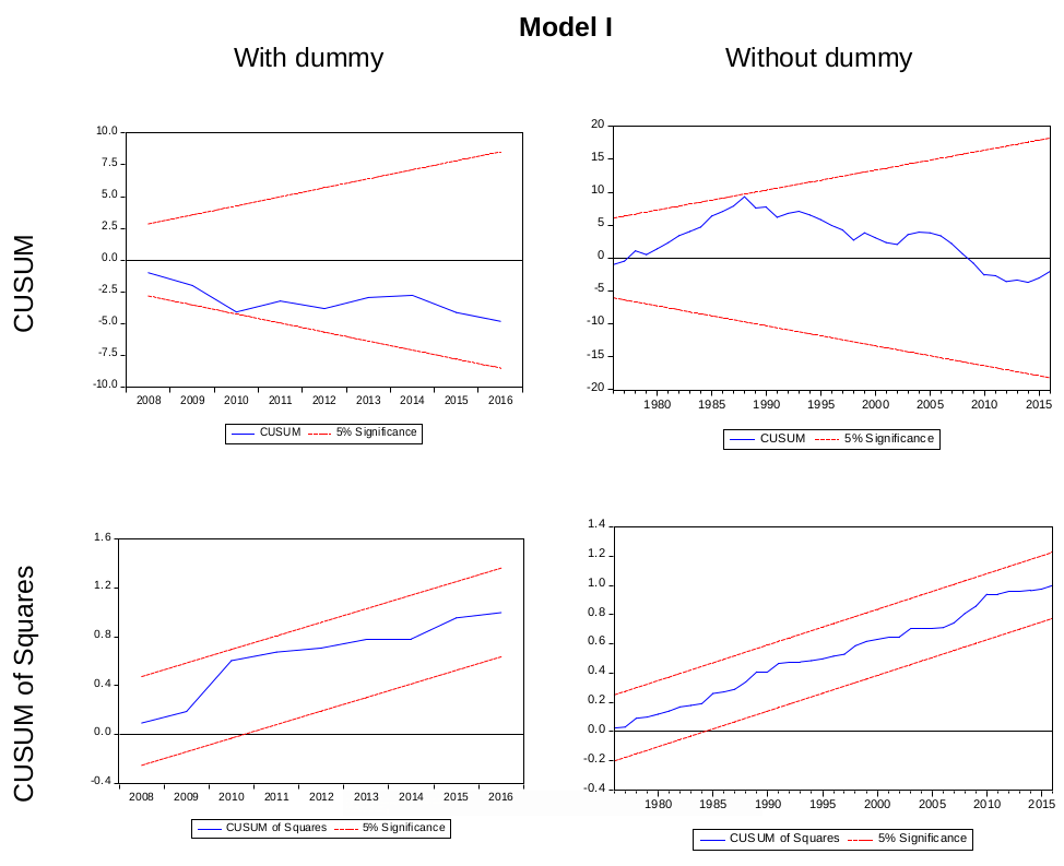
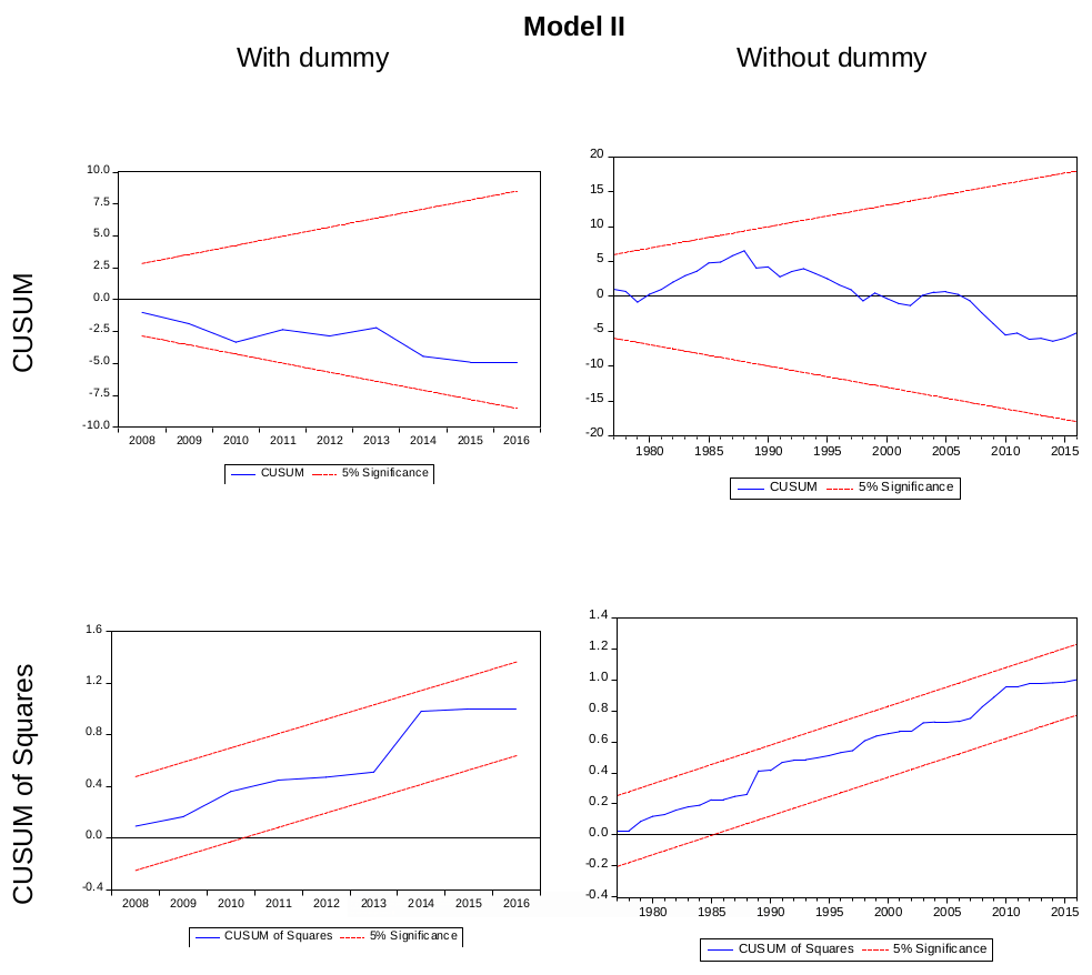
Finally, the stability of the parameters was verified through CUSUM and CUSUM of Squares test. Details in figure 2.
Figure 2 – CUSUM and CUSUM of Squares.
|
|
Source: Author’s elaboration.
Through the graphs, it is concluded that the parameters are stable, in the presence or absence of dummies, since the CUSUM and CUSUM of Squares lines are within the significance of 5%.
The ARDL results are robust and are in line with the results presented in the pairwise structure. In the long-run, in models I and II, all independent variables impact the dependent variable (DLPC). In the short-run just DLPC(-1), DLGDP, DPOPG and DPOPG(-1), it has an impact on gambling expenses.
In both models, shift-type dummies were introduced to control the subprime mortgage crisis (SMC) effect. For the model, I, the dummy is from 2007 to 2014. For model II, the dummy is from 2007 to 2013. They are reinforcing that the impacts of the crisis were global and also affecting the gambling industry. Others researches that focus on gambling, during this period, should incorporate this break to avoid econometric instability.
The misery index and its decomposition (UN and INFL) have high explanatory power over the dependent variable in the long-run. The phenomenon that the index of misery captures relates to the well-being and wealth of the population. In the event unemployment and inflation cause society to lose its purchasing power, increase the sensitivity of economic instability and suggests an induction to the game, which can be a way to “change lives”.
In the short-run, a 1% increase in GDP induces an increase in gambling expenditure by over 1%. In a model, where the economy is growing, even at a slow rate, it brings a feeling of security to the population, which enables a higher proneness to risk. In the long-run, if economic stability exists and is assimilated by society and a higher level of risk is also found, meaning that a positive and meaningful impact on the gambling industry.
The models showed a positive coefficient for the delayed dependent variable (DLPC (-1)). That means that past spending has an impact in the same direction in the present. It can be concluded that the dependent variable is autoregressive, a result corroborating with Livingstone et al. (2018) on the nature of the variable and its effects. In addition to reinforcing the existence of absolute dependence on the game. This result further contributes to the debate on the adverse effects of the game (e.g. Nichols & Tosun, 2017; Davis et al., 2017).
An increase in the population of 1% would cause at a long-run an increase in gambling expenditure over 2%. The results of population growth are indicative of an economy growing. However, in short-run, the positive and negative variations are distinguishable. Suggesting that the same endogenous factors that drive population growth also increase gambling expenses.
The SMC (2008-09) had a crucial limiting impact on the gambling industry. There is evidence of the depressing impact of the economic crisis on gambling expenditure (e.g. Horváth & Paap, 2012; Gu, 1999). Horváth & Paap (2012) stated that in challenging economic scenarios, excessive consumption decreases. Gambling consumption, from an economic point of view, is a superfluous one, as such, is sensitive to the economic crisis. However, the cases of compulsive players require attention because they are not linear.
The results show that the classic version of the misery index has a substantial impact on gambling expenditure in the long-run. The data appears to indicate that a decrease in well-being would lead society to become more prone to risk. Individuals would find gambling as a form of improving their standard of living. That is possible due to some types of gambling requiring low amounts of money, a small percentage when compared to possible earnings (e.g. Mikesell, 1994).
According to the laws of the United States, all forms of gambling are age-restricted (18-21 years usually considered the minimum ages), this factor is a possible explanation of the higher impact of population growth in the long-run. Individuals need to reach a certain age to access all forms of gambling legally.
Regarding economic income (measured recurring to GDP) a higher level of wealth would enable the populations to gamble more. Thus, explaining the positive impact of this variable in the long-run. The results suggest two interactions, tourist expenditure, international and national. This interpretation was due to the knowledge that a closed economy cannot grow; there would only exist capital redistribution. Which corroborates what Li et al. (2010) stated that gambling enterprises could not grow if their client base is entirely local, it is of the utmost importance that the industry can attract foreign gamblers/visitors, for it is the only way towards growth.
The model revealed that in the long-run, electricity consumption has a substantial adverse impact on the gambling (in models I and II, the impact is: -3.631531 and -3.663492, respectively). One of the causes we suggest is that technological development has produced new forms of entertainment that also act as substitutes for gambling. The contrast between different generations can also be seen in entertainment patterns. Younger generations are more comfortable to use with new technologies, which consequently use electricity as a source of energy.
Are online games (with or without financial risk) the substitutes for the standard form of gambling? The access to this type of entertainment is not always free. For access, there is a need for proper payment, in addition to the obligation to have more equipment to use. Indeed, it requires access to new technologies, streamlines processes and facilitates of communication. However, different generations of users have diverse preferences. Genc (2014) points out that children beg to play with smartphones and tablets. We also see incentives for younger people to be included in the design processes to develop new technology solutions for children’s users (Chimbo & Gelderblom, 2018).
Historically, the industry has been capable of evolving (Horváth & Paap, 2012), and became a centre for entertainment, while always looking to expand their customer base (e.g. restaurants, commercial centre, showroom, hotels, etc.). This new situation is just another opportunity for development. Casinos have detected this crisis and have been developing forms of gambling more appealing to newer generations, such as the introduction of video games/skill-based games in casino floors. The state of Nevada has even introduced new legislation to accommodate this new form of gambling. This study further strengthens the necessity for the industry to be able to adapt to the changes in customs and beliefs of the populations.
5 - CONCLUSION
This research analyses the impact of wealth and poverty on gambling expenditure. To achieve this objective, we recurred to the ARDL method. The study focuses on the United States, and the annual data ranges from 1965 to 2016. The hypotheses of this article have been validated. Wealth and poverty (inflation and unemployment or misery index) are positively related to gambling expenses, and new forms of gambling can negatively affect the gambling industry.
The new forms of gambling could be proxied, albeit crudely, by the consumption of electricity. The results show that this variable exerts a reductive impact on gambling expenses in the long-run. That is, without an effort by gambling companies to innovate and develop their services, the American gambling industry can put some of their profits at risk.
During the subprime mortgage crisis, there is a decrease in gambling expenditure. Overall, wealth (measured by GDP) is pro-cyclical with gambling expenditure, means that it follows the economic situation. One of the suggestions that can be made after analysing the results is when looking to the increase of state revenues. Gambling can be a solution to maximise states’ income during boom periods. For the gambling industry does not to be a zero-sum game, it is essential that public policies and the incentives for tourism being carefully thought out. Political barriers can undermine this vital source of income in the state.
Gambling is a phenomenon influenced by much more than only psychological factors. The results of this research also indicate that economic factors are necessary to explain the expenses with gambling. At the state or city level, a microeconomic analysis can provide public and private decision-makers with valuable information that could benefit their economic policies.
CKNOWLEDGEMENTS
The financial support of CEFAGE - Center for Advanced Studies in Management and Economics, sponsored by the FCT - Portuguese Foundation for the Development of Science and Technology, Ministry of Science, Technology and Higher Education, project UID/ECO/04007/2019, is acknowledged. The financial support of NECE - Research Unit in Business Science and Economics, sponsored by the FCT - Portuguese Foundation for the Development of Science and Technology, Ministry of Science, Technology and Higher Education, project UID/GES/04630/2019, is acknowledged.
REFERENCES
AGA (2017). Casino industry essential to small business growth. Available in:https://www.americangaming.org/newsroom/press-releasess/new-study-casino-industry-essential-small-business-growth. Accessed on 10/27/2017.
Adhikari, B. K., & Agrawal, A. (2016). Religion, gambling attitudes and corporate innovation. Journal of Corporate Finance, 37, 229-248. doi: 10.1016/j.jcorpfin.2015.12.017.
Ahmad, Y., & Mykhaylova, O. (2017). Exploring International Differences in Inflation Dynamics. Journal of International Money and Finance. 79, 115-135. doi: 10.1016/j.jimonfin.2017.09.002.
Akee, R. K., Spilde, K. A., & Taylor, J. B. (2015). The Indian gaming regulatory act and its effects on American Indian economic development. The Journal of Economic Perspectives, 29(3), 185-208. doi: 10.1257/jep.29.3.185.
American Psychiatric Association. (Ed. 5). (2014). DSM-5: Manual Diagnóstico e Estatístico de Transtornos Mentais. Porto Alegre: Artmed. (pp. 585-590). ISNB 978-85-8271-088-3.
Ayllón, S., & Ferreira-Batista, N. N. (2017). Unemployment, drugs and attitudes among European youth. Journal of Health Economics, in Press. doi: 10.1016/j.jhealeco.2017.08.005.
Barbieri, C. (1999). Educação pelo esporte - Algumas considerações para a realização dos Jogos do Esporte Educacional. Movimento. 5(11), 23-32. ISSN: 0104754X.
Barro, R. J. (1999). Reagan vs. Clinton: Who’s the Economic Champ? Business Week, 22(5).
Bernstein, P.L. (Ed.). (1996). Against the Gods: The remarkable story of risk. John Wiley & Sons, New York.
Beyerlein, K., & Sallaz, J. J. (2017). Faith’s wager: How religion deters gambling. Social Science Research, 62, 204-218. doi: 10.1016/j.ssresearch.2016.07.007.
Chang, T., & Chen, W. Y., (2017). Revisiting the relationship between suicide and unemployment: Evidence from linear and nonlinear cointegration. Economic Systems, 41(2), 266-278. doi: 10.1016/j.ecosys.2016.06.004.
Chimbo, B., & Gelderblom, H. (2018). TitanTutor: An educational technology solution co-designed by children from different age groups and socio-economic backgrounds. International Journal of Child-Computer Interaction. 15, 13-23 doi: https://doi.org/10.1016/j.ijcci.2017.11.004
Choi, B., Park, W., & Yu, B. K. (2017). Energy intensity and firm growth. Energy Economics, 65, 399-410. doi: 10.1016/j.eneco.2017.05.015.
Dadayan L, Ward R. B. (2009). For the first time, a smaller jackpot: Trends in state revenues from gambling. Albany: The Nelson A. Rockefeller Institute of Government.
Davis, A. K., Bonar, E. E., Goldstick, J. E., Walton, M. A., Winters, J., & Chermack, S. T. (2017). Binge-drinking and non-partner aggression are associated with gambling among Veterans with recent substance use in VA outpatient treatment. Addictive Behaviors, 74, 27-32. doi: 10.1016/j.addbeh.2017.05.022.
Dolan, P., Peasgood, T., & White, M. (2008). Do we really know what makes us happy? A review of the economic literature on the factors associated with subjective well-being. Journal of Economic Psychology, 29(1), 94-122. doi: 10.1016/j.joep.2007.09.001.
Donayre, L., & Panovska, I. B. (2018). US Wage Growth and Nonlinearities: The Roles of inflation and Unemployment. Economic Modelling. (68), 73-292. doi: 10.1016/j.econmod.2017.07.019.
Drydakis, N., (2015). The effect of unemployment on self-reported health and mental health in Greece from 2008 to 2013: A longitudinal study before and during the financial crisis. Social Science & Medicine, 128, 43-51. doi: https://doi.org/10.1016/j.socscimed.2014.12.025.
Dumitrescu, E.I., & Hurlin, C. (2012) Testing for Granger non-causality in heterogeneous panels. Economic Modelling, 2012, 29.4: 1450-1460.
Fiedler, I., Kairouz, S., Costes, J.M. & Weißmüller, S. K. (2019) Gambling spending and its concentration on problem gamblers. Journal of Business Research, 98, 82-91. doi: http://10.1016/j.jbusres.2019.01.040
FRED (2017). Total Gross Domestic Product for Las Vegas-Henderson-Paradise, NV (MSA). Available in:https://fred.stlouisfed.org/series/NGMP29820. Access in 10/27/2017.
Fuinhas, J. A., & Marques, A. C. (2012). Energy consumption and economic growth nexus in Portugal, Italy, Greece, Spain and Turkey: an ARDL bounds test approach (1965–2009). Energy Economics, 34(2), 511-517. doi: 10.1016/j.eneco.2011.10.003.
Fuinhas, J. A., & Marques, A. C. (2013). Rentierism, energy and economic growth: The case of Algeria and Egypt (1965–2010). Energy policy, 62, 1165-1171. doi: 10.1016/j.enpol.2013.07.082.
Fuinhas, J. A., Marques, A. C., & Carreira, R. (2015). A different look over the financial depth nonlinearity: Evidence from Europe. Revista de Estudos Sociais, 17(35), 120-135. ISSNe 2358-7024.
Genc, Z. (2014). Parents’ perceptions about the mobile technology use of preschool aged children. Procedia-Social and Behavioral Sciences, 146, 55-60. doi: 10.1016/j.sbspro.2014.08.086.
George, S., Velleman, R., & Nadkarni, A. (2017). Gambling in India: Past, present and future. Asian journal of psychiatry, 26, 39-43. doi: 10.1016/j.ajp.2017.01.018.
Goh, S. K., Sam, C. Y., & McNown, R. (2017). Re-examining Foreign Direct Investment, Exports, and Economic Growth in Asian Economies Using a Bootstrap ARDL Test for Cointegration. Journal of Asian Economics. doi: 10.1016/j.asieco.2017.06.001.
Granger, C.W.J. (1969). Investigating causal relations by econometric models and cross-spectral methods. Econometrica, 37 (3), pp. 424-438
Green, F. (2011). Unpacking the misery multiplier: How employability modifies the impacts of unemployment and job insecurity on life satisfaction and mental health. Journal of Health Economics, 30, 265-276. doi: https://doi.org/10.1016/j.jhealeco.2010.12.005.
Gu Z. (1999). The Impact of the Asian financial crisis on Asian gaming activities: An examination of Las Vegas strip casino drops. Current Issues in Tourism. 2(4), 354–365. doi: 10.1080/13683509908667861.
Gu, X., & Tam, P. S. (2011). Casino taxation in Macao: An economic perspective. Journal of Gambling Studies, 27(4), 587-605. doi: 10.1007/s10899-010-9235-8.
Gu, X., Li, G., Chang, X., & Guo, H. (2017). Casino tourism, economic inequality, and housing bubbles. Tourism Management, 62, 253-263. doi: 10.1016/j.tourman.2017.04.006.
Guo, Z., Robinson, D., & Hite, D. (2017). Economic impact of Mississippi and Alabama Gulf Coast tourism on the regional economy. Ocean & coastal management, 145, 52-61. doi: 10.1016/j.ocecoaman.2017.05.006.
Hofer, V., & Leitner, J. (2011). Should European gamblers play lotto in the USA? European Journal of Operational Research, 215(1), 181-187. doi: 10.1016/j.ejor.2011.05.049.
Horváth, C., & Paap, R. (2012). The effect of recessions on gambling expenditures. Journal of Gambling Studies, 28(4), 703-717. doi: 10.1007 / s10899-011-9282-9.
Howarth, R. B., & Kennedy, K. (2016). Economic growth, inequality, and well-being. Ecological Economics, 121, 231-236. doi: 10.1016/j.ecolecon.2015.10.005.
Jalil, A., Mahmood, T., & Idrees, M. (2013). Tourism–growth nexus in Pakistan: Evidence from ARDL bounds tests. Economic Modelling, 35, 185-191. doi: 10.1016/j.econmod.2013.06.034.
Kahneman, D., Krueger, A. B., Schkade, D., Schwarz, N., & Stone, A. A. (2006). Would you be happier if you were richer? A focusing illusion. Science, 312(5782), 1908-1910. doi: 10.1126/science.1129688.
Katrakilidis, C., & Trachanas, E. (2012). What drives housing price dynamics in Greece: New evidence from asymmetric ARDL cointegration. Economic Modelling, 29(4), 1064-1069. doi: 10.1016/j.econmod.2012.03.029.
Kovács, I., Richman, M., Janka, Z., Maráz, A., & Andó, B. (2017). Decision making measured by the Iowa Gambling Task in alcohol use disorder and gambling disorder: A systematic review and meta-analysis. Drug and Alcohol Dependence 181(1), 152-161. doi: 10.1016/j.drugalcdep.2017.09.023.
Lai, T. M., To, W. M., Lo, W. C., Choy, Y. S., & Lam, K. H. (2011). The causal relationship between electricity consumption and economic growth in a Gaming and Tourism Center: The case of Macao SAR, the People’s Republic of China. Energy, 36(2), 1134-1142. doi: 10.1016/j.energy.2010.11.036
Li, G., Gu, X., & Siu, R. C. S. (2010). The impacts of gaming expansion on economic growth: A theoretical reconsideration. Journal of Gambling Studies. 2010;26(2):269–285. doi: 10.1007/s10899-009-9165-5.
Li, J. S., Alsaed, A., Hayat, T., & Chen, G. Q. (2014). Energy and carbon emission review for Macao’s gaming industry. Renewable and Sustainable Energy Reviews, 29, 744-753. doi: 10.1016/j.rser.2013.09.001.
Livingstone, C., Adams, P., Cassidy, R., Markham, F., Reith, G., Rintoul, A., Schüll, N. D., Woolley, R., & Young, M. (2018). On gambling research, social science and the consequences of commercial gambling. International Gambling Studies, 18(1), 56-68. doi: 10.1080/14459795.2017.1377748.
Lovell, M. C., & Tien, P. (2000). ECONOMIC DISCOMFORT AND CONSUMER SENTIMENT. Eastern Economic Journal, 26(1), 1-8. jstor.org/stable/40325964.
Marques, L. M., Fuinhas, J. A., & Marques, A. C. (2017). Augmented energy-growth nexus: economic, political and social globalization impacts. Energy Procedia 136, 7-101. doi: https://doi.org/10.1016/j.egypro.2017.10.293.
Mills, D. J. & Nower, L. (2019) Preliminary findings on cryptocurrency trading among regular gamblers: A new risk for problem gambling?. Addictive Behaviors, 92, 136-140. doi: http://10.1016/j.addbeh.2019.01.005
McMillen, J. (Ed.). (2005). Gambling cultures: Studies in History and Interpretation. Routledge. (pp. 6). ISBN 1134916485, 9781134916481.
Mikesell J. L., (1994). State lottery sales and economic activity. National Tax Journal. 47(1), 165–171. ISSN: 0028-0283.
National Gambling Impact and Policy Commission (US). (1999). The National Gambling Impact Study Commission Final Report. Available in: https://www.ncjrs.gov/App/Publications/abstract.aspx?ID=182780 Access in: 08/01/2018.
Nichols, M. W., Tosun, M. S., & Yang, J. (2015). The fiscal impact of legalized casino gambling. Public Finance Review. 43(6), 739-761. doi: 10.1177/1091142115574900.
Nichols, M. W., & Tosun, M. S. (2017). The impact of legalized casino gambling on crime. Regional Science and Urban Economics. 66, 1-15. doi: 10.1016/j.regsciurbeco.2017.05.005.
Nucera, F. (2017). Unemployment fluctuations and the predictability of currency returns. Journal of Banking & Finance. 84, 88-106. doi: 10.1016/j.jbankfin.2017.07.007.
Özcan, S. E., & Açıkalın, S. (2015). Relationship between Misery Index and Lottery Games: The Case of Turkey. International Journal of Humanities and Social Science, 5(7), 159-164. ISSN 2220-8488.
Pesaran, M. H., Shin, Y., & Smith, R. J. (2001). Bounds testing approaches to the analysis of level relationships. Journal of applied econometrics, 16(3), 289-326. doi: 10.1002/jae.616.
Rahman, M. M., & Kashem, M. A. (2017). Carbon emissions, energy consumption and industrial growth in Bangladesh: Empirical evidence from ARDL cointegration and Granger causality analysis. Energy Policy, 110, 600-608. doi: 10.1016/j.enpol.2017.09.006.
Rahman, M. S., Noman, A. H. M., & Shahari, F. (2017). Does economic growth in Malaysia depend on disaggregate energy? Renewable and Sustainable Energy Reviews, 78, 640-647. doi: 10.1016/j.rser.2017.05.010.
Ramoni-Perazzi, J., & Orlandoni-Merli, G. (2013). El índice de miseria corregido por informalidad: una aplicación al caso de Venezuela. Ecos de Economía, 17(37). ISSN 1657-4206.
Sek, S. K., (2017). Impact of oil price changes on domestic price inflation at disaggregated levels: Evidence from linear and nonlinear ARDL modeling. Energy, 130, 204-217. doi: 10.1016/j.energy.2017.03.152.
Shahzad, S. J. H., Nor, S. M., Ferrer, R., & Hammoudeh, S. (2017). Asymmetric determinants of CDS spreads: US industry-level evidence through the NARDL approach. Economic Modelling, 60, 211-230. doi: 10.1016/j.econmod.2016.09.003.
Shin, Y., Yu, B., & Greenwood-Nimmo, M. (2014). Modelling asymmetric cointegration and dynamic multipliers in a nonlinear ARDL framework. In Festschrift in Honor of Peter Schmidt (pp. 281-314). Springer New York. doi: 10.1007/978-1-4899-8008-3_9.
Simcock, N., & Mullen, C. (2016). Energy demand for everyday mobility and domestic life: Exploring the justice implications. Energy Research & Social Science, 18, 1-6. doi: 10.1016/j.erss.2016.05.019.
Van den Bergh, J. C. (2009). The GDP paradox. Journal of Economic Psychology, 30(2), 117-135. doi: 10.1016/j.joep.2008.12.001.
Walker, D. M., & Jackson, J. D. (2011). The effect of legalized gambling on state government revenue. Contemporary Economic Policy, 29(1), 101-114. doi: 10.1111/j.1465-7287.2010.00198.x.
World Bank (2019). World Development Indicators. Disponible in: https://databank.worldbank.org/data/reports.aspx?source=2&series=NY.GDP.MKTP.KN&country=#. Access in: 10/02/2019.
APPENDIX